I’ve used Ceph several times in projects where I needed object storage or high resiliency. Other than using VMs, it’s never something I can easily run on at home to test, especially not on bare-metal. Circa 2013, I tried to get it running on a handful of Raspberry Pi Bs that I had, but they had far too little RAM to compile Ceph directly on, and I couldn’t get Ceph compiling reliably on a cross-compiler toolchain. So I moved on with life. Recently, I’ve been looking at Ceph as a more resilient (and expensive) replacement for my huge file server. I found that it’s now packaged on Arch Linux ARM’s repos. Perfect!
Having that hurdle out of the way, I decided to get a 3 node Ceph cluster running on some Raspberry Pis.
My plan is to have each node run all of the services needed for the cluster. This isn’t a recommended configuration, but I only have three Raspberry Pis to dedicate to this project. Additionally, I’m using a fourth Raspberry Pi as an automation/admin device, but it isn’t directly participating in the cluster.
Putting it all Together:
Create a master image to save to the three SD cards. I grabbed the latest image from the Arch Linux ARM project and followed their installation directions to get the first card set up.
Note: I used the Raspberry Pi 2 build, because the Ceph package for aarch64 on Arch Linux ARM is broken. I’m also using 13.2.1, because Arch’s version of Ceph is uncharacteristically almost a year old and I wasn’t going to try to compile 14.2.1 myself again.
Once the basic operating system image was installed, I put the card into the first Raspberry Pi and verified that SSH and networking came up as expected. It did, getting a static IP address from my already configured DHCP server.
I first tried to use Chef to configure the nodes once I got them running. Luckily Arch has a PKGBUILD for chef-client in the AUR. Unluckily, it’s not for aarch64. Luckily again, Chef is supported on aarch64 under Red Hat. I grabbed the PKGBUILD for x86_64, modified it to work with aarch64, built and installed the package.
I created a chef user, gave it sudo access, generated an SSH key on my chef-server, and copied it to the node.
At this point, I had done as much setup on the single node I had, so I copied the image onto the other two microSD cards, and put them into the other Pis.
Chef expects to be running on a system that isn’t Arch Linux. After some time trying to get it working, I decided that I’d spent enough time trying to get it working.
With Chef a bust, I moved on to Ansible and re-imaged the cards to start fresh.
ceph-ansible initially worked better, due to Ansible being supported on Arch Linux, but the playbook doesn’t actually support Arch. I needed to make some modifications to get the playbook to run.
With some basic configuration of the playbook ready to go, I got the mons up and running pretty easily. But osd creation failed on permissions issues. Something in the playbook was expecting a different configuration that Arch Linux uses. Adding the ceph user to the “disk” and “storage” groups partially fixed the permissions issues, but osd creation was still failing. Ugh.
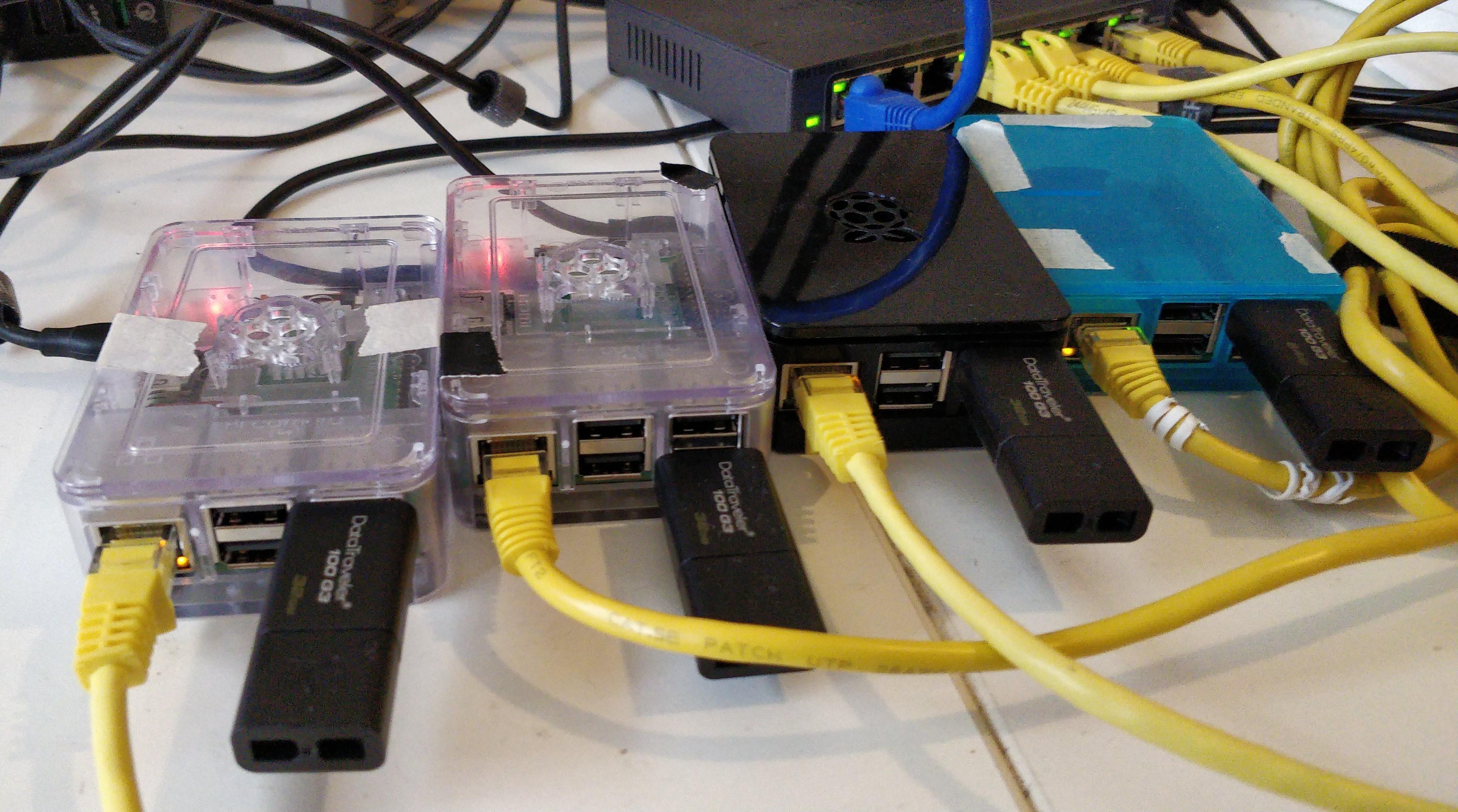
Ceph cluster in operation. The rightmost blue Raspberry Pi is being used as an admin/automation server and isn’t part of the actual Ceph cluster.
Time for Manual Installation:
While part of my goal was to try some of the Ceph automation, chef’s and ceph-ansible’s lack of support for Arch Linux meant that I wasn’t really accomplishing my main goal, which was to get a small Raspberry Pi cluster up and running.
So I re-imaged the cards, used an Ansible bootstrap playbook that I wrote and referred to Ceph’s great manual deployment documentation. Why manually deploy it when ceph-deploy exists? Because ceph-deploy doesn’t support Arch Linux.
MONs:
MONs or monitors stores the cluster map, which is used to determine where to store data to meet the reliability requirements. They also do general health monitoring of the cluster.
After following all of the steps in the Monitor Bootstrapping section, I had the first part of a working cluster, three monitors. Yay!
One difference from the official docs, in order to get the mons starting on boot, I needed to run systemctl enable ceph-mon.target in addition to the ceph-mon daemons, otherwise systemctl listed their status as Active: inactive (dead) and they didn’t start.
MGRs:
The next step was to get ceph-mgr running on the nodes with mons on them. The managers are used to provide a interfaces for external monitoring, as well as a web dashboard. While Ceph has documentation for this, I found Red Hat’s documentation more straight forward.
In order to enable the dashboard plugin, two things needed to be done on each node:
First, run ceph dashboard create-self-signed-cert to generate the self-signed SSL certificate used to secure the connection.
Then run ceph dashboard set-login-credentials username password, with the username and password credentials to create for the dashboard.
Running ceph mgr services then returned {"dashboard": "https://rpi-node1:8443/"}, confirming that things had worked correctly, and I could get the dashboard in my browser.
OSDs:
Now for the part of the cluster that will actually store my data, the OSD, which use the 32GB flash keys. If I wanted to add more flash keys, or maybe even hard drives, I could easily add more OSDs.
I followed the docs, adding one bluestore OSD per host on the flash key. One note, as I’d already tried to set the keys up using ceph-ansible, they did have GPT partition tables. I ran ceph-volume lvm zap /dev/sda on each host to fix this.
Additionally, I didn’t realize that the single ceph-volume command also sets up the systemd service, and I created my own. Now I had an OSD daemon without any storage in the cluster map. I followed Ceph’s documentation and removed the OSD, but now my OSDs IDs start at 1 instead of 0.
MDSs:
I plan on testing with CephFS, so the final step is to add the MetaData Server, or MDS, which stores metadata related to the filesystem. The ceph-mds daemon was enabled with systemctl enable ceph-mds@rpi-nodeN (N being the number of that node) and then systemctl enable ceph-mds.target so that the MDS is actually started.
Now What?
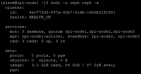
A healthy Raspberry Pi Ceph cluster, ready to go.
The cluster can’t store anything yet, because there aren’t any pools, radosgw hasn’t been set up and there aren’t any CephFS filesystems created.
If I had more Pis, I’d love to test thing with more complex CRUSH maps.
The next blog post will deal with testing of the cluster, which will likely include performance tuning. Raspberry Pis are very slow and resource constrained compared to the Xeon servers I’ve previously run Ceph on, so I expect things to go poorly with the default settings.
SimCity 2000 is the second of Maxis’ well received city builders and is my favourite in the series, in addition to being one of my favourite games of all time. I’m not sure exactly why, but it’s the best blend of building and management and the art.
I found that SimCity 4 was all about micromanagement at a scale that wasn’t fun. The game was too hard, at least without mods to fix some of the more serious issues. SimCity 2000’s art style is very well done 8-bit graphics which I knew weren’t supposed to be hyper-realistic and never looked janky, unlike some of the later games. Maybe there’s also some nostalgia too.
Despite being released around a quarter-century ago as of this writing, I still play the game occasionally. I play the Windows 95 version, which is the definitive version. Unfortunately, it doesn’t run on modern versions of Windows without a patch to the executable, so the inferior DOS version is the only one commercially available presently.
Even when I was a child, playing the game, I’d often get to the (admittedly large for the time) limits of the 128×128 tile map and wish my city could somehow continue past it, but actually doing so was beyond my abilities then.
I’d built one city out of 25 individual tiles over several years during high-school and early University, painstakingly reconciling the edges as I went. It was slow going, and I eventually got tired of it as it was getting to be more and more work as it grew.
A city I called Thomnar, which doesn’t mean anything, that I built using 5×5 city tiles.
And then in 2014, I was finishing up my last semester of University and working, and I felt the draw to the game again. I still really liked that large, multi-tile city and wanted to work on it more, but reconciling the edges was annoying. Except this time, I had the tools and technical ability to start reverse engineering the game and working on a re-implementation.
My initial goal was simple: figure out the city binary file format and write something to automatically reconcile the edges.
As I figured out more and more of the format, my focus shifted from writing a tool to reconcile edges to a complete re-implementation of the game. This also involved figuring out the complete sprite file spec, as well as working on the text data files.
Having the (nearly) complete city file spec also means that I can make cities that are impossible to make in the game, such as this city that is floating in the clouds.
I have gotten most of the .sc2 file spec figured out, all of the game sprite file spec as well as the .mif sprite spec and some of the text file specs done, which are kept up-to-date on my GitHub.
I also have written a Python library and related tools to open, edit and save out the modified .sc2 file, available under my reverse engineering project on GitHub: OpenCity2k.
I use two cameras for my mobile livestreaming setup for birding. I’ve got one wide camera, that I mainly use as I walk to show the general area, and a zoom camera that I used to focus in on a specific bird. I can switch between the two cameras, and sometimes I also want to display both.
I get asked to how it works, so I figured I’d write a high-level blog post on how it works, without getting into the nitty-gritty specific details.
Here’s an example, with some debug overlays enabled. The zoom camera is the main view, with the inset being the wide view of the area I’m birding in.
As I primarily stream from Nvidia Jetson devices, I’ll focus on those, but the following should be adaptable to anything that supports gstreamer and some sort of compositor (preferably hardware accelerated if on a SBC like the Jetsons).
Software Used
There are two main ingredients to make this all work: gstreamer and gst-interpipe. I use gstd to make things easier to automate.
Gstreamer is obvious, it’s required to run everything. gst-interpipe is used to split the pipelines into different pieces. I’ve structured things as a pipeline for each of the inputs, a pipeline for the compositing and a pipeline for the encoding and output. Why not split each input into it’s own pipeline, with audio and video separate? I had some strange audio/video synchronization issues with each in their own separate pipelines, and found that having them in the same pipelines kept their timestamps consistent with each other.
gstd is just a daemon that wraps gstreamer pipelines and allows them to be accessed by an API. I chose it because I didn’t want to get bogged down in writing code in C/C++ to use gstreamer directly.
The Pipelines
This is an example of an input pipeline for a V4L2 video device with an Alsa audio device. In this case, it captures raw (uncompressed) video and audio from a UVC capture device. There would be two of these inputs for two capture devices, and these inputs could be just audio or video. They needn’t be a V4L2 source either, they could be an srtsrc, rtpsrc or any other source that gstreamer supports. If the input is encoded, then it will need to be decoded to raw in the input pipeline. Each input needs a unique name property on the interpipesink.
I have found that putting the audio and video inputs in the same pipeline can help with synchronization issues that sometimes crop up. Note that Nvidia’s compositor doesn’t seem to like mixed framerates, so there is an explicit videorate to keep it happy. There isn’t any reason why all of these pipelines couldn’t all be put in one pipeline, but I split them in up for better separation of concerns.
Next comes the compositor. In this example, there are two 1080p sources, with one resized to be 480 x 270 (1/4th 1080p) as a picture-in-picture (PiP) inset, located in the bottom left corner. The compositor works on RGBA only, so there’s an nvvidconv step to convert the two inputs to RGBA. On a non-Jetson system, this would be accomplished using the videoconvert and compositor elements (or similar).
And finally, the encoder block. In this case, it’s encoding the video to HEVC (H265) and the audio to Opus. The video and audio is then muxed to MPEG-TS and finally sent over the network using SRT. In this case, the audio is the first input, and the video is the output of the compositor.
The “magic” in the switching is being able to dynamically link interpipesink elements to interpipesrc elements. Simply change the listen-to property on the interpipesrc to change inputs. If compositing (PiP) isn’t needed, the compositor pipeline can be omitted and the encoder/muxer/transmitter pipeline can be directly manipulated to switch inputs. With the compositor, the inset and main source can be swapped by changing the interpipesink each interpipesrc listens to.
Changing the layout of the compositor is similar, but takes more steps. Each property on each compositor sink needs to be changed. Care needs to be taken to make sure that the inset’s zorder property is a higher number than the main image, otherwise it’ll end up hidden. This is particular to gstd, as code using gstreamer directly can change more than one property at once.
There’s also no reason why more inputs can’t be used. A Jetson Nano, for instance, can do 4 simultaneous inputs, depending on the input. Simply add more input pipelines and more sinks to the nvcompositor, and set the properties appropriately.
Updates
07-Feb-2024: I made a small copy-paste error in one of the gstreamer pipelines, this has been fixed. I also made a couple edits/clarifications based around questions and feedback.
With the header sorta figured out, and unit data partially figured out, there’s still a lot more file that hasn’t been determined yet.
Immediately after the last floor’s unit information, the game does a 4 Byte read, followed by some number of 16 Byte entries. As I quickly suspected, the number of entries is exactly the same as those 4 Bytes interpreted as an integer. Perfect, now we at least know the structure of another large chunk of the file.
Next Parts
But what do we do with this? First I started by dumping the values into a terminal to see if I could see any patterns. Two things jumped out at me, the first and third values increment. The first goes up from 0 to 113, which is the count of floors in the building that have anything on them (including the cathedral’s multiple stories above floor 100). So we’ve got one entry per floor, it seems. Some floors seem to have no entries, which appear to be lobbies or otherwise completely empty floors.
Next, I started looking for a pattern in the number of entries on a floor and what’s on that floor. Quickly, I saw that there were 30 entries for floors with 10 condo units on them. This suggests a condo has 3 entries. Knowing the game, I know that a condo has a population of 3 people, so these must be entries related to people!
Checking a floor with 19 offices there are 114 entries. Offices have 6 people per office, so that’s what this data structure is for. On to the contents of the data structure, past the two that were immediately apparent. The next pattern I spot in that the second byte is also incrementing, and seems to be the index of the unit on the floor. Now we’ve got 3 / 16 Bytes figured out. What’s next?
I name a couple people and use the in game tools to find them throughout the building, and see that byte 7 seems to be the current floor they’re on, and byte 5 looks suspiciously like bit-flags, even if I don’t know what exactly they mean yet. They may show things like if a person is in the building or not, sleeping, etc. I think the last four bytes are two 16 bit integers, and these may be storing the stress and eval(uation), but these don’t look consistent.
What’s After People?
I decide to put the people data aside and see what’s next. The ProcMon CSV (explained in Part 1) shows a read of 9,216 Bytes, with no read for length before it. This suggests to me that this is a static sized block. It’s divisible by 16, but 576 isn’t a nice “round” number, not like 512. Seeing that this is close to 512, I try the next larger even number. 9,216 / 18 is 512. There’s our nice round number.
From this, I can strongly infer that I’m dealing with a fixed length of 512 entries, each 18 bytes in size. Maybe they have a similar structure to our unit structure, which also has an 18 byte size. I can also see that not all of them are full from a hex editor. Where else do I have a similar number? I know the count of commercial (shop, restaurant, fast-food place, etc.) is 419. I’m betting that I’ll have 419 complete values, and the rest as empty placeholders/padding. Let’s see. I’ve included the some entries in the section, with their decimal values shown.
One of the things I do with values is stick them in a dictionary to see what sorts of results I get, and how many.
# commercial_list is a list of "unparsed" commercial objects, which is just the list of values above.
values = [defaultdict(int) for _ in range(18)]
for comm in commercial_list:
#    if comm.values[0] == 255:  # uncomment to skip empty floors
#        continue
    for i in range(18):
        values[i][comm.values[i]] += 1
# And then a quick and dirty print to see the results.
for i, e in enumerate(values):
    print(f"{i} ({len(e)}):")
    print(', '.join([f"{k}: {v}" for k, v in e.items()]))
# Or sorted with values only, and not counts. Equivalent to using a set().
    print(', '.join([str(k) for k in sorted(e.keys())]))
I’m not going to include the full output but I can quickly see a few things. Most evident is that value for the first byte the values range from 1 to around 100, which suggests that this is a floor number. Except several entries are FF (=255), and these are otherwise empty. How many non-empty values do we have? 419! Yep, this is additional metadata related to commercial tenants, separate from the data in the Units data. Likely this stores their profits, eval, etc. Given that we know the floor now, lets see what else we can find out.
I can also see that the 15th, 16th and 18th (last) bytes are 0, at least in this test tower. I see that byte 3 only has the values 0, 1, 2 and 3. Knowing other things about the game helps me look for other values. I know there are 5 fast food places. 5 restaurants and 11 different shops. None of the bytes has 21 different entries, but the 12th byte has 11 entries, ranging from 0 to 10. Perhaps this is the index of which variant, which is supported by there being many more entries with 0-4, than than other 6 values, which are nearly identical. So I think this byte is the unit’s variant.
How do I check this easily? I used my thumbnail generation code from before and made thethe unit look up its entry in the commercial data section by its index, and then use the variant to choose a colour. In this case, I generated 11 different HSV colours, converted to RGB and used those. From this, I can see indeed this is the variant, and from looking at the game, I can see what each value refers to.
But something is wrong. That red block on the bottom left? Those three aren’t all the same, so something is going on here. This looks overall correct, but it seems that order things were built in matters. There doesn’t look like pointers back to the in the Commercial Data Section, and there isn’t anything in the Unit data structure. But there’s that 188 Bytes for each floor. I divide 188 by 4, but 47 isn’t a number that means much in SimTower. 188 by 2 is 94, which is much more interesting. 375 (the width of a floor) tiles / 4 tiles for the smallest unit (a single hotel room or parking stall) gives 93.75 maximum units on a floor. So, maybe that 188 bytes is a 2 byte count, and up to 93 remapping pointers?
Doing them in order allowed me to figure out the indices, but now I have the issue that they’re not correctly re-mapped. So how does the re-mapping table work? There isn’t a initial count byte, so it looks like there are 94 possible 2-byte counts here.
After trying to figure out the mapping, I decided to move on, but will revisit the section. It’s tantalizingly close, but having more entries in it than units on a floor, as well as repeated entries, suggests that it’s not as straight forward as I’d hoped.
Elevator Data
Next thing in the data we have is a repeated data structure composed of a 194 Byte read, a 480 Byte read, two 120 Byte reads and then up to 29x 324 Byte reads and up to 8x 346 Byte reads. This was all repeated 24 times for a building full of elevators. The game allowing only 24 elevators is a well known limitation, so this is clearly all of the elevators.
Normal and service elevators can be 29 floors tall and have a maximum of 8 cars, so this these segments likely store that information about an elevator shaft. Further confirmation that this is indeed elevators. For a tower with fewer than 24 elevator shafts, only the 194 Byte header exists, so somewhere inside this block is metadata related to height. 120 Bytes is probably 120 flags related to floors.
Looking at a building full of elevators, I can see that a maximum height elevator has 29 of the 324 Byte entries and minimum height elevator has 1. I can also see that the last 8 bytes in the header are an elevator car’s home floor, with the value being the start floor of the elevator if those cars don’t exist.
Further investigation reveals a count of cars, starting tile from the left the elevator is on, and the top and bottom floors. But what did I do to figure this out? I made a change, such as adding another car or changing the elevator height to see what changed.
Sure looks like elevators. Black is normal elevators, red is service and blue is express elevators. Express elevators have a little different format. They only have a floor data structure for each floor that can stop at, not all of the floors they cover. This is likely because in the game, they only stop on underground floors, and at floors 1, 15, 30, 45, 60, 75, and 90 (which all can be sky-lobbies).
From there, the only other data in the header that isn’t determined yet is a 56 byte segment in the middle. There appear to possibly be 4 sub-sections that are 14 bytes each. One segment of is all 5, which is the default number of floors for an elevator car to service. Which means that this is storing the configuration of the elevator scheduler in the elevator properties window. Changing the settings confirms this, but there are only 6 periods to configure. This could mean that there’s a 7th hidden period, or more likely in my opinion, this was changed at some point in development.
With that figured out, the elevator header is done. But what about the next 480 bytes, or the two sections of 120 bytes? Those look suspiciously like information about floors. What happens if we take the info and assign every 4 numbers a colour and generate a 4 x 120 byte image for the 480 byte segment? This could be a status indicator of some sort for each car, so perhaps we need to split into 8x 4 bit values. Let’s see what that looks like too.
he first two entries show an express elevator going from floor B9 to 90, and the second shows a normal elevator going from floor 75 to 100. The left column represents a “legend” showing underground floors in a bluish colour, lobbies in a greenish colour and unused “floors” at the top in a reddish colour with the next column always black.
That certainly looks like it has something to do with elevator car statuses. But what exactly? The values don’t seem to match those shown in the elevator’s status section, but there is definitely a pattern there. I see repeated patterns at lobby floors, as well as underground (but not on B10, which can only be used for the Metro line’s tunnel). But also similar patterns between the express elevator and the normal elevator, especially where they overlap. Is this from people on those floors wanting to get somewhere? Something else? I’m still not sure, but being able to visualize data like this really helps.
Moving on, next I looked at the 324 byte floor data segment. The first thing I notice is that 324 bytes would be an even 80 entries of 4 Bytes, plus a single 4 Byte header, and this is exactly what this structure looks like. I could see that the values looked exactly like IDs in the people data segment. Closer inspection indicated that after the header, there are two independent segments. I noticed this because on the bottom floor of the elevator, one half was completely empty, with the same being true of the other half on the top floor. On floors not serviced, both were empty. But what about the header? It looks like 4 single byte values? A quick look at the game showed that the first and third values were the number of people waiting on the left and right of the elevator, or going up and down, respectively, and that this count capped at 40.
With the elevator data mostly sort-of decoded, I decided to move on to the next segments. I’m getting close to the end of the file, so there isn’t a whole lot else. I’m expecting data for the finance window, stairs and escalators and similar, though perhaps some of this is stored in that 490 Byte block at the beginning that I skipped.
The Next Segments
I can see a read of 88 bytes, of 132 bytes, of 12 bytes and of 42 bytes. SimTower does use 32 bit integers is some places, but the game is still really a 16 bit game, so even in places the save uses 32 bit integers to store the data, the numbers never get that large. This means that something that looks like XX XX 00 00 in the game file is usually a giveaway to interpret this as a 32 bit integer. The first and second entries look like this, while the third and fourth don’t.
The second entry has numbers that match the finance window, so that’s easily decoded.
I got sidetracked while looking at that segment, and I found that the next segment, at 1026 bytes long, had an initial value that was what looked like a 2 byte count, and then an increasing index up to that count. I looked at what else shared that count, and it was the number of parking stalls in the tower. So this stores some information related to the parking stalls. Once I got past the basic structure, which appears to be a count of connected stalls, verified by removing a stall and seeing that the count of stalls with red ‘X’s in them was subtracted here, the rest appeared to be a 2B index value. However, once I removed and added a stall, and checked, the values got a bit weird, so I’m not sure what this does.
Next comes a 22 Byte long block, which is mostly empty, so maybe this is padding or a placeholder?
After that comes 64x 10 Bytes blocks. There are 64 elevators and escalators in the game, so that’s what’s stored here, as there isn’t much else left in the file, and I haven’t found it anywhere else yet.
Looking at the actual structure, the first byte is 01 if there’s a set of stairs of escalator built, and the second appears to indicate what is built. Interestingly, 0 is escalator, so maybe they were added first. There are 6 total values for the each of the stair and escalator variants, total. The next two bytes are the same for all the stairs/escalators in one test tower, and it appears to be how far from the left side it is. The next byte is the start/bottom floor, though this is potentially two bytes.
The next set of two bytes, or single byte and second padding/other byte, appears to be the count of people going up and down the escalator respectively. How did I figure this out? Well, I guessed that the number of people shown in the game must be stored somewhere, and like the elevator cars, the total number of people should be stored inside this segment. But I had an escalator with 14 people on it, and I didn’t see 14. After staring at it a bit, I realized that 9 and 5 equal 14. Sure enough, this value matched on all the stairs and escalators I checked. I figured out the direction by looking at the counts first thing in the morning just after the fast food places opened, and people were only going up from my floor 1 lobby, via escalators, to them.
Final Bits
After the escalator/stairs section are 8 segments of 484 Bytes each. This looks suspiciously like a 4-Byte header, and 120 entries afterwards, one for each floor. Each entry might be a 4B value, but it could also be 4x 1B or 2x 2B. I didn’t have much luck decoding this one, other than to note that the first 4 Bytes are a header, because it’s a specific value if the rest of the entry is empty, and that the 120 values don’t look like 4 Byte integers. I’ll need to poke at this some more, but it looks like something that maybe isn’t exposed directly in the game and is instead internal simulation related.
Next are 10x 2Byte entries. My first thought it security offices, as there are a maximum of 10 of these. There are also a maximum of 10 medical clinics, but security offices are treated differently by the game, so it makes sense that these would be noted separately, even though they’re stored in the Units Data section as well. And sure enough, each value if either -1 or the floor that a security office is built on.
There’s still some more sections to go, I see a bunch of 6 Byte long entries, 10x 4 Byte entries (medical clinics), 16x 12 Byte entries, a 80 Byte entry, a 40 Byte entry. After that are three entries that seem the same length in a few towers I looked at, which are a 4,354 Byte entry, 2,114 Byte entry and a 3,234 entry. I have no idea what these store, but it’s probably more internal simulation state as a cursory inspection didn’t really reveal any structure, but a more thorough investigation may show something.
At the very end, there’s an 8 Byte read (of what seems to be empty data) and then 16B entries for named entities in the game. I’m not entirely sure how the entries are mapped, but the first entries are for named units, and the rest are for named people in the tower.
Ending Thoughts
I was very quickly able to determine most of the overall structure of the file, but things got more difficult towards the end of the file where there were lots of blobs that weren’t structured in a way that made their usage apparent.
My approach of figuring out the reads the game was doing and then looking at the data those reads contained really helped. I’ve looked at newer games that just load the entire file into memory and parse it, and they’re much more annoying to reverse engineer.
I’ve also poked at reverse engineering other games that I was less familiar with, and knowing things like there can only be 512 commercial units in a building really helped when I had a section that was a multiple of that length long.
There’s still a lot to be determined, and lots of unknown values sprinkled in the documentation, but overall, I got a large proportion of the file format figured out. As was the case for my SimCity 2000 city format reverse engineering project, the first 90% takes 10% of the time, and the remaining 10% takes 90% of the time.
I’ll need to decide whether or not I’m interested in grinding out more of the documentation on the format, but the documentation is open source on GitHub, so other people can always use it as a basis and open pull requests if they discover something new. But there are still parts I skipped that seem like they’d be relatively easy to do, so I’ll probably do some more work on this before I set it aside for whatever my next project it.
Or I’ll start a re-implementation project of the game. No guarantees…
Another game from my childhood that I played a lot was SimTower. Never to the same extent as SimCity 2000, but still a fixture of my game playing time. Note that I’m writing this as I work on the reverse engineering, and I plan to update with more information on my process.
Someone in a Discord was commenting that they would like to see a viewer (and maybe editor) like the one I’ve created for SimCity 2000. I decided to take a crack at the .TDT (Tower DaTa?) format SimTower uses to store the towers, especially given I’ve got a decent amount of experience reverse engineering old game formats like what SimTower uses.
First Steps
The first step was to get the game working. I found that Winevdm worked pretty well, but I needed to copy WAVEMIX.INI from my CD into Winevdm’s WINDOWS folder, and WAVEMIX.DLL into WINDOWS\SYSTEM in order for the game to start. With that out of the way, the game started.
Now, one of the tools I used to help reverse engineer the .SC2 file format was ProcMon, because old games frequently loaded small chunks of the save file into memory, likely to save on relatively limited RAM resources as they may be stored in a more RAM efficient data structure when in use, and serialized to something that’s better for that (or not).
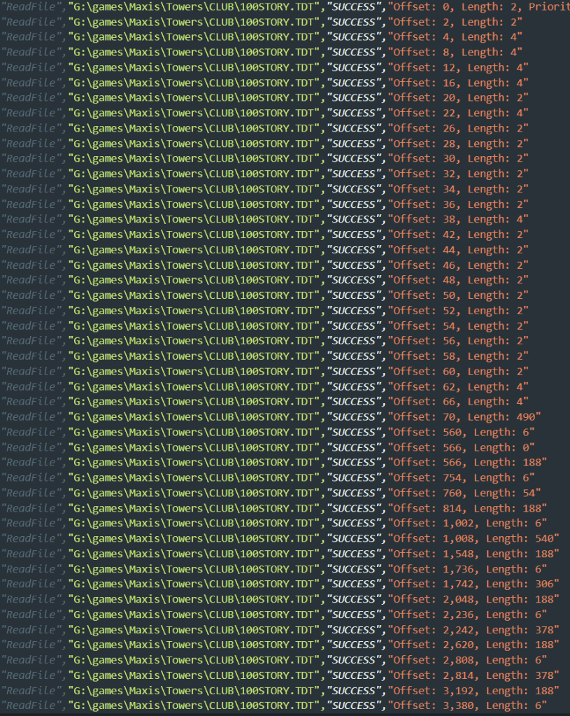
SimTower was luckily no different, giving me my first hints as to what the file format looks like. I’ve attached a CSV output from ProcMon, as an image from VSCode so that it’s a little nicer coloured below.
Part of the CSV output of ProcMon after filtering. “ReadFile” means that it’s reading a file, the next part is the path to the files and “SUCCESS” means the read was successful and returned data. But the interesting part is the offset into the file and the length. The small, short reads are generally indicative of reading value in single variable. The repeated pattern is also really interesting, as it suggests repeated entries of the same data structure.
Floor Data
Immediately I can pick out a few things. The first 70 bytes look like a header, because it was common for games of the time to load various single variables individually, especially if they store counts or lengths of later values. Inspecting the value of a few towers confirms this is probably the case. I’ll touch on the header later. There also seems to be another 490B block common in most tower files I looked at. Past that, there’s a suspicious repetition of 360 reads following the same format. 6 Bytes, variable bytes and 188 Bytes.
Note: The game save is little-endian, so data will be in reverse order of Big-endian, which I’m more used to on x86 systems. This probably means the game was originally developed for the Mac and ported. In this case, I looked at the hex representation of several of the 4 Byte values, and saw XX YY 00 00, which is the ordering I’d expect for a small number stored little-endian. Bit-endian would be `00 00 YY XX` instead, with the unused data on the left and the byte order reversed.
As a guess, 360 reads means 120 actual values. SimTower has at least 113 floors (10 underground, 100 normal floors and a additional 3 floors for the cathedral on the 100th floor), so a few extra to pad out the window to 120 seems reasonable. I also note that each variable length piece is always a multiple of 18 Bytes long, so my first guess is that each of these is a “unit” on a floor.
The 6 Bytes repeated screams “row header” to me, and after creating a tower with 110 floors, save the first floor lobby, of empty floors, I see my first pattern. I know, from counting money spent building a full width floor, that I have 375 horizontal tiles to work with. In my empty tower, each of the 6 Bytes looks like 01 00 00 00 77 01 which interpreted as 3 integers is 1, 0, 375. Given that the floors cover the whole width, the second and third value appear to be the start and end of the floor. Inspecting several other saves confirms this, and I also noticed a pattern in the first value. It’s the count of the number of 18B entries after it.
Which means yes, we’ve got floor data here. There’s still a lot of data that isn’t accounted for. People’s and business’ nicknames (the game allows setting name for people and businesses, and this appears to be stored at the end of the file), elevators, various simulation variables, etc.
Unit Data
Now that we know, at minimum, a unit is given by an 18Byte structure, we can start sussing that out. Right away, I see that my empty tower has one unit, and the data structure mirrors the 6 Byte header, with the first 4 Bytes being 00 00 77 01 followed by 00 or 24 for my height 1 lobby, which suggests that this is a unit type field.
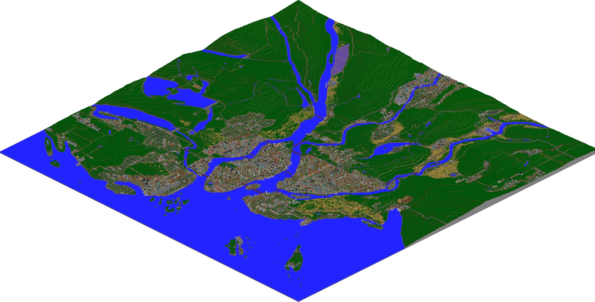
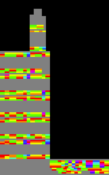
If I know start and end of a floor, as well as start and end of a unit and the unit’s type, then I can start figuring out what values in the field correspond to the type in the game. Rather than squint at a blast of text in a proof-of-concept Python parsing script, I decided to write a simple image generator using Pillow. Here’s an example of a 5 star tower I built to test things out.
A 100 story tower with empty space in blue, lobbies in purple, yellow for shops, grey for fast food, green for restaurants, salmon and cyan for hotel rooms, turquoise for offices, brown for condos and other colours for other things. Referring between this and the game is easy to figure out the index mapping.
And just like that, with randomly chosen colours, we can see a tower take shape. The smallest “block” in SimTower is a 10×45 pixel tile (or so), so I made each block 1×5 pixels in this image to maintain a similar aspect ratio. Immediately I can see the blank space (blue), various commercial units, the lobbies, the Metro station (3 stacked colours in the bottom right, as well as the Metro tunnel at the very bottom), the Cathedral’s 5 stories at the top and various other units. This allowed me to get quickly the values for the rest of the various units for the type, because I could just look at them in the game.
Looking at this simple graphic can also be useful to figure out what other data parts of the data structure mean. For example, here’s another one. For those who play the game, can you guess what the various colours mean?
Pricing modeled after the in-game map/overlay. Default is “average” pricing, or yellow. High is red, low is green and very low is cyan. The top part was set for testing, but I had some shops stubbornly empty due to low traffic unless I dropped the pricing.
It’s game pricing of the units. Yellow is average price, red is high, green is low and cyan is very low. I set these colours after I figured it out, to mirror what was in the game, but it made visually figuring out that part of the data structure very easy.
Others can be more perplexing, such as this one showing a specific unknown value in the Unit data structure for shops. Perhaps this is an index somewhere else, as the values look largely unique. But being able to see data like this makes finding patterns so much easier.
Unknown data, with each entry coloured a random colour, or gray for the build foorprint of the tower.
Header Data
Okay, but now what about that header? Here I use another debugging tool, CheatEngine, to inspect the running memory of the game. While CheatEngine may be designed to allow cheating at games, I’ve almost exclusively used it as a debugging tool, as there are that many easy debugging tools with a similar feature set on Windows.
Unlike SimCity 2000, which had a normal start address, SimTower running under Winevdm made for a little more work. But not much. I started by looking for the values in the save file, saving the game a couple times and scanning for the new value in CheatEngine. Quickly I found that the first value was the tower’s rating (SimTower towers start at 1 star and progress through 5 stars to finally receive a tower rating) by opening towers with different ratings. I also saw that the values in the save, without using CheatEngine for some of the other values referred to money and budgetary values (the game displays the money values multiplied by $100, but would store that as 1).
I played the game and watched the values change, quickly finding a value tracking number of commercial units (fast-food, restaurant and shops), one for parking stalls, one for recycling facilities, one for security facilities as well as a few others. As of when this was written, I don’t have them all figured out.
One thing I noticed looking is that the game runs with a various number of ticks per second of in game time. The one hour period between Noon and 1:00PM has 800 ticks out of a total of 2600 ticks for the whole day associated with it. Meanwhile, between 1:00AM and 7:00AM only has 200 ticks of simulation time. When I was playing the game as a child, I assumed that was just because there was more to simulate during the day, not that the game had lower fidelity simulations then. I guess lunch time being exceptionally busy is a 90’s Japanese office-worker thing that I was never exposed to. This also means that the day starts at 7:00AM, at least as far as the game is concerned, because this is when the tick counter rolls over.
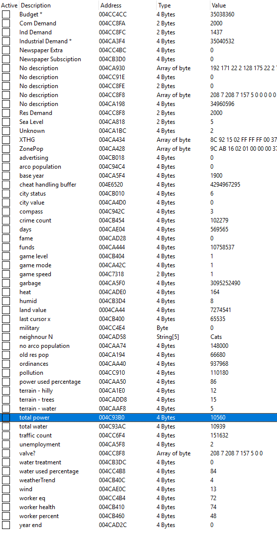
I’ve attached the whole 70 Byte header in CheatEngine with a 5-star tower with $115,300,900 in cash, paused, to show what various values look like. I added the labels myself after I figured them out, or noted it as unknown. Note that the addresses shown are likely not going to be the same after an app restart.
Final Thoughts
I got a lot more done a lot quicker than I expected, likely because I’ve spent quite a bit of time getting good at this specific sort of reverse engineering from the SimCity 2000 reverse engineering project. I’ve started a GitHub repo with my findings here, and includes my sample parsing code in all it’s gory glory. It’s quick, dirty, and gets the job done.
I’ll write a part 2 as I work on the rest of the file. Elevators and a bunch of other information still need to be determined, and I’d like to share more about the more fiddly aspects of reverse engineering, but this post is enough for tonight.
The Ceph cluster is continuing to run fine and generally meets all of my needs, though I could definitely use more IOPs, especially for RBD volumes attached to VMs. I have encountered a couple operational issues that may crop up in a home environment outside a datacenter with redundant internet connectivity and power. If you’d like to read more on the cluster hardware choice, setup and testing, you can here.
Timekeeping
I had a nearly 3-day Internet outage caused by a Telus’ general sloppiness. While I was offline, my cluster wasn’t able to keep time using NTP. While I had the cluster computers pulling NTP from a local NTP server (running on my PFSense router), all of its sources of time were on the Internet, except that derived from its onboard clock. At some point, NTP on the Ceph servers decided that the upstream was bad, and so dropped it. Over a day the clocks on the servers drifted enough that Ceph started having serious issues. I ended up needing to shut down the cluster, and with it, all the VMs using it for storage, because it had degraded to the point of being unusable due to how Ceph handles clock skew. Luckily, I had a USB based GPS unit handy, and I was able to set myself up a backup stratum 1 NTP server using the GPS and a Raspberry Pi. While USB GPS units generally have significantly more jitter than serial ones due to the vagaries of USB’s timing, it was much lower than the clocks on the servers, and this satisfied Ceph.With higher quality timekeeping my cluster was back to being healthy and able to serve writes. I ended up using GPSD to access the GPS and Chrony to handle being the NTP server. I found this guide and this one useful to get things working.
Lessons learned: Time synchronization is important for a healthy Ceph Cluster. Have a local backup time source. While Ceph can be tuned to be more tolerant to poor time sync, there’s no replacement for stable time infrastructure.
Power
A month or so after the Internet outage, I had a power outage that lasted 1.5 hours. My backup power for the cluster has about 75 minutes of runtime, so the cluster was shut down. I powered down the VMs and then set the following flags on the cluster (source):
ceph osd set noout
ceph osd set nobackfill
ceph osd set norecover
To bring the cluster back, I started the three hosts back up and unset the flags. However, when everything came back up, I realized that I hadn’t waited enough time before powering down the hosts, and some of the VM’s RBD disks hadn’t finished syncing. Cue several hours of running xfs_repair on a bunch of RBD devices. In the end, I didn’t lose any data, just had lightly corrupt filesystems.
Lessons learned: Safe shutdown needs to be handled automatically, with attention taken to how the cluster is being used. I wrote a safe shutdown script to use with Proxmox and apcupsd that shuts down the VMs, calls sync twice and then waits a (hopefully very conservative) 10 minutes before powering off the hosts, to ensure that all data has been properly written to disks. As my hosts are not set to power back on when power comes back, I’m manually un-setting the flags when the system come up.
Memory
I also learned that 64GB of memory was not enough to run Ceph and VMs on the same hosts, as Ceph could easily use 40+GB of RAM on its own, leading to RAM exhaustion of the hosts. I upgraded to 128GB of RAM by adding another of the same kit to each host, which is the maximum amount the board and CPU supports.
I’m still having issues with RAM exhaustion under heavy load of VMs and CephFS, so it seems like 265GB of RAM may actually be a good idea, but that’s out of my budget. I was seeing Ceph using 80+GB of RAM under heavy CephFS metadata workloads, which was a backup operation determining if files had changed since the last backup. My general fix has been to better spread VMs across hosts and to limit how many metadata operations I’m putting through CephFS at once.
Other Tweaks
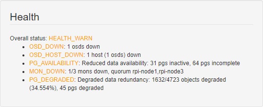
Sometime I was getting Ceph into HEALTH_WARN with showing OSDs with slow ops, and dmesg was full of errors like nvme nvme0: I/O 42 QID 47 timeout, completion polled. This appears to be due to a firmware bug in the Intel P4510 SSDs I’m using, that has since been fixed. So I did some baseline tests and then updated the firmware on the hosts and rebooted.
Download the Intel Memory and Storage Tool (MAS), CLI version for Linux from Intel’s website. Strangely, Proxmox doesn’t have this packaged (licensing issues).
Unzip it.
Install the debian package using apt install ./intelmas_<version>_amd64.deb.
Find the SSD using MAS: intelmas show -intelssd
Update the firmware: intelmas load -intelssd <SSD #>.
Reboot
This update tripled the I/O throughput of the nvme-only pool residing on the SSDs, both in IOPs and raw bitrate. Maximum latency, as reported by sysbench went from 30 seconds to 90 milli-seconds. And, no more errors in dmesg or slow ops on my OSDs. Incidentally, this performance increase was triggering the OOM conditions mentioned in the previous section, due to the increased performance needing more RAM.
Conclusion
I’m still pretty happy with Ceph at home, but there are certainly some considerations that crop up with home use that don’t in a datacenter, though they should probably also be planned for even with redundant power and connectivity, in the event of a true disaster.
Below is my current cluster usage. I’ve got a 37TiB CephFS filesystem running on it, with the remainder being used for RBD images for VMs and the like.
I’ve always wanted to use Ceph at home, but triple replication meant that it was out of my budget. When Ceph added Erasure Coding, it meant I could build a more cost-effective Ceph cluster. I had a working file-server, so I didn’t need to build a full-scale cluster, but I did some tests on Raspberry Pi 3B+s to see if they’d allow for a usable cluster with one OSD per Pi. When that didn’t even work, I shelved the idea as I couldn’t justify the expense of building a cluster.
When my file-server started getting full, I decided to build a Ceph cluster to replace it. I’d get more redundancy, easier expansion and have refreshed hardware (some of my drives are going to be 9 years old this summer). I briefly looked at ZFS. But between its limited features and with the legality of running it on Linux being an open question, I quickly ruled it out.
The Cluster – Hardware
Three nodes is the generally considered the minimum number for Ceph. I briefly tested a single-node setup, but it wasn’t really better than my file-server. So my minimal design is three nodes, with the ability to add more nodes and OSDs if and when my storage needs grow.
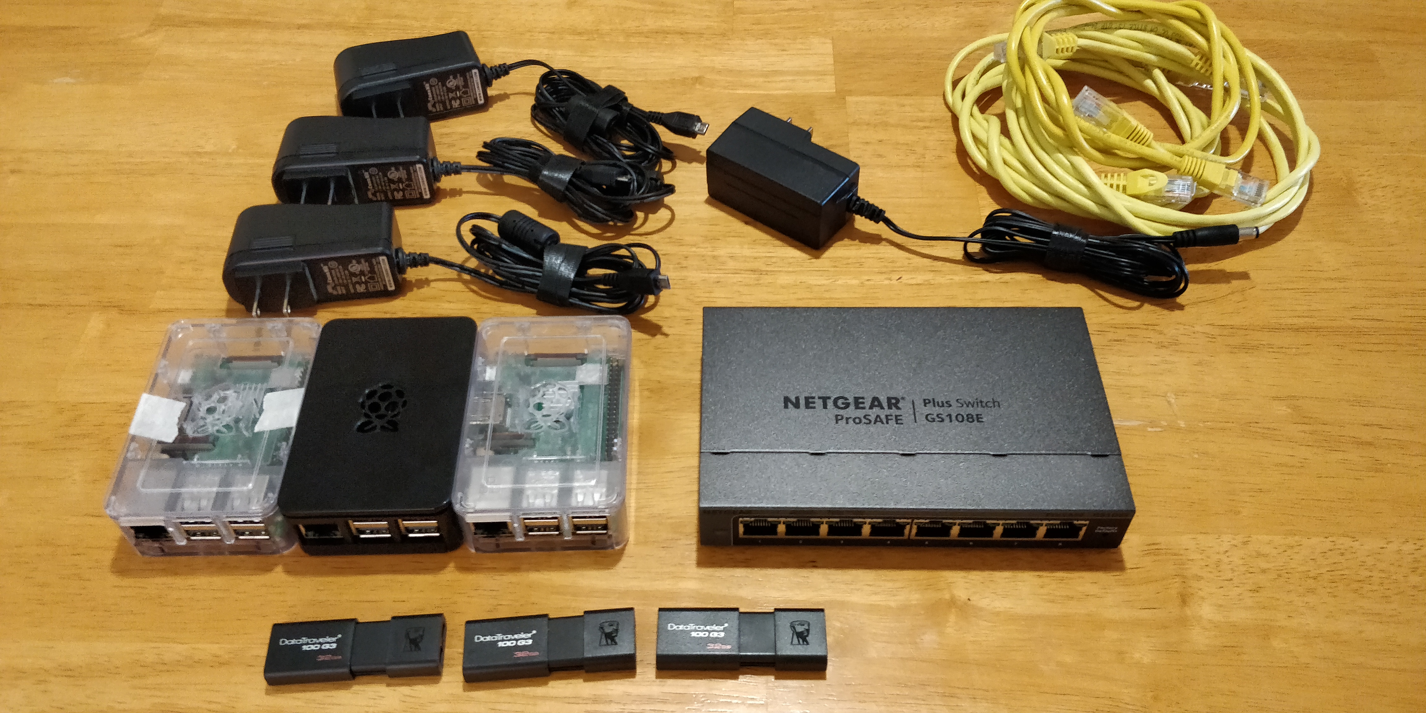
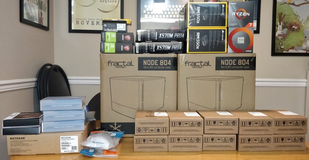
Some of the hardware waiting to be built into cluster nodes sitting on my dining room table. Not pictured is the first node I built for a single-node test.
I wanted each node to be small and low-ish power, so I was mainly looking at mATX cases that could take 8 3.5″ drives. After much searching, I realized that mATX is basically dead and there aren’t many mATX cases or motherboards out there. Presumably people either get mITX cases and motherboards if they want something small or get full ATX boards if they want lots of on-board peripherals and expandability, leaving mATX as an awkward middle ground.
For the motherboard, it needed to have (either onboard or space to add via add-in cards): 8xSATA (or SAS), 2x M.2 (at least one 22110) slots, 8-core CPU (or better), support for 32GB RAM sticks and a single 10GbE port (not SFP+). I found three boards that would work, a SuperMicro board that was incredibly expensive but had everything except the CPU onboard, an AMD X570 based board and an Intel Z390 based board. I quickly ruled out the SuperMicro board based on price and the Intel board based on the lack of low-power CPUs (to get the 8-cores, I was looking at a 9700k, which isn’t low-power or particularly fast or the 9900T, which no one could get me). I chose an ASRock X570M Pro4 board. It had what I needed, and better yet, it supported a 65W, 8-core Ryzen 3 CPU. I’d been bit by serious hardware bugs in the Ryzen 1, so I was a bit wary to try it, but Intel had nothing anywhere near competitive.
HDD choice was relatively easy, I created a spreadsheet with all the drive models I could find, found the best $/TB 7200RPM model I could. This ended up being 6TB Seagate Ironwolf drives, which were discontinued in favour of an inferior model after I ordered mine. Luckily with Ceph, replacements don’t need to be the same size like they did in RAID6.
SSDs were a little more challenging. I chose inexpensive, but good, M.2 SSDs for the OS drives. I also wanted some SSD based OSDs. Ceph apparently does not do well on consumer level SSDs without power-loss-protection and consequently has very slow fsync performance, so I needed a fancier SSD than the Samsung 970 Pros I had been intending to use. I found the Intel P4510/P4511 series, and decided on a 2.5″ U.2 P4510. This required an M.2 to min-SAS adapter and mini-SAS to U.2 adapter to get it connected to the board’s open M.2 slot. Why not use the P4511? No stock on it.
Part
Count
Notes
Fractal Design Node 804 – Case
3
8×3.5″, 2×2.5″, mATX, full ATX PSU
ASRock X570M Pro4 – Motherboard
3
mATX, 8xSATA, 2x M.2, PCIe4.0 x16, x1, x4
Corsair RM550x – Power Supply
3
ATX PSU
Seagate 6TB Ironwolf – Hard Drive
18
OSD: 6 per node, 108TB Raw, ST6000VN0033
Kingston SC2000 250GB – M.2 SSD
3
OS/Boot Drive
Intel P4510 1TB – U.2 SSD
3
OSD: 1 per node
AMD Ryzen 3700x = CPU
3
65W, 8-core
64GB Corsair LPX – RAM
3
One 2x32GB DDR4 3200 per node
Geforce GT710 – Video Card
3
One per node
Startech M.2 to U.2 Adapter Board
3
To connect P4510 SSD to motherboard
Mini-SAS to U.2 Adapter Cable
3
Cable to connect from Startech adapter to SSD
4x SATA Splitter Cable
6
One per each bank of 4 drives, 2 per node
Corsair ML120 120mm 4-pin fan
3
One each on front of drive compartment
Aquanta AQ-107 – 10GbE NIC
3
One per node
Cat 6a Patch Cable
3
One per node
Netgear 8-port 10GbE Switch
1
Model: XS708E, one for the whole cluster
Cluster hardware.
A small note on networking: I elected not to have separate public and cluster networks, I set everything to use the same 10GbE network. This simplified setup, both on the host/Ceph as well as physical cabling and switch setup. For a small cluster, the difference shouldn’t matter.
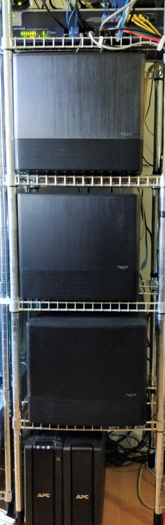
Three cluster nodes in an Ikea Omar wire rack. At the bottom is a 1500VA APC UPS with a 3kVA additional battery. At the top is my core switch, and the cluster’s 10GbE switch.
Other hardware notes: the Fractal Design Node 804 HDD mounts are missing one of the two standard screw holes. The spec for 3.5″ drives only requires the two end holes, but the Node 804’s mounts only support the optional middle hole and the hole nearest the connectors. Most drives 6TB and over lack the middle hole, apparently to allow another platter.
The Cluster – Setup
Setup was pretty straightforward. I used Arch Linux as a base, running Ceph version 14.2.8 (then current). I installed the cluster using the Manual Deployment instructions.
Once the cluster was running, it was time to create pools and set up the CephFS filesystem I planned on migrating to. Ceph correctly assigned my hard drives as hdd class and the SSDs as ssd class. I had planned to have CephFS backed by an erasure coded pool, with a durability requirement of being able to lose either two drives or one host (but not both). CephFS doesn’t allow EC coded pools to be used to the CephFS metadata store, so I created a replicated pool on the P4510 SSDs. I’m using the P4510s to store the metadata because suggestions online were that it would increase performance to have the metadata pool on SSDs. I’m not sure if this actually makes much difference with the low number of drives I have.
I created a CRUSH rule that will place data only on SSDs with: ceph osd crush rule create-replicated ssd-only default host ssd.
To make sure this CRUSH rule worked, I tested it by:
Dumping a copy of the crushmap using ceph osd getcrushmap -o crushmap.orig
Running crushtool --test -i crushmap.orig --rule 2 --show-mappings --x 1 --num-rep 3 (the number after --rule is the index of the rule to test). Results: CRUSH rule 2 x 1 [18,20,19], which are the OSD numbers of my SSDs, exactly as intended.
Finally, create the pool with ceph osd pool set cephfs-metadata crush-rule-name ssd-only. Excellent! On to the EC pool.
Three Node Cluster – EC CRUSH Rules
The EC coded pool took a little more work to get working. My design goal is to have the cluster be able to suffer the failure of either a single node or two OSDs in any nodes. To do this, I would minimally need to split each block up into four pieces, plus two parity pieces.
What the OSD tree looks like:
$ ceph osd tree
ID CLASS WEIGHT    TYPE NAME          STATUS REWEIGHT PRI-AFF
-1       100.97397 root default
-3        33.65799     host Alecto
 0   hdd   5.45799         osd.0          up  1.00000 1.00000
 1   hdd   5.45799         osd.1          up  1.00000 1.00000
 2   hdd   5.45799         osd.2          up  1.00000 1.00000
 3   hdd   5.45799         osd.3          up  1.00000 1.00000
 4   hdd   5.45799         osd.4          up  1.00000 1.00000
 5   hdd   5.45799         osd.5          up  1.00000 1.00000
20   ssd   0.90999         osd.20         up  1.00000 1.00000
-5        33.65799     host Megaera
 6   hdd   5.45799         osd.6          up  1.00000 1.00000
 7   hdd   5.45799         osd.7          up  1.00000 1.00000
 9   hdd   5.45799         osd.9          up  1.00000 1.00000
11   hdd   5.45799         osd.11         up  1.00000 1.00000
14   hdd   5.45799         osd.14         up  1.00000 1.00000
16   hdd   5.45799         osd.16         up  1.00000 1.00000
19   ssd   0.90999         osd.19         up  1.00000 1.00000
-7        33.65799     host Tisiphone
 8   hdd   5.45799         osd.8          up  1.00000 1.00000
10   hdd   5.45799         osd.10         up  1.00000 1.00000
12   hdd   5.45799         osd.12         up  1.00000 1.00000
13   hdd   5.45799         osd.13         up  1.00000 1.00000
15   hdd   5.45799         osd.15         up  1.00000 1.00000
17   hdd   5.45799         osd.17         up  1.00000 1.00000
18   ssd   0.90999         osd.18         up  1.00000 1.00000
I found a blog post from 2017 describing how to configure a CRUSH rule to make this happen, but that post was a little light on how to actually do this.
Get a copy of the existing crushmap: ceph osd getcrushmap -o crushmap.orig
Decompile the crushmap to plaintext to edit: crushtool -d crushmap.orig -o crushmap.decomp
Edit the crushmap using a text editor. This is the rule I added:
rule ec-rule {
        id 1
        type erasure
        min_size 6
        max_size 6
        step set_chooseleaf_tries 5
        step set_choose_tries 100
        step take default class hdd
        step choose indep 3 type host
        step choose indep 2 type osd
        step emit
}
Some explanation on this rule config:
min_size and max_size being 6 is how many OSDs we want to split the data over.
step take default class hdd means that CRUSH won’t place any blocks on the SSDs.
The lines step choose indep 3 type host and step choose indep 2 type osd tell CRUSH to first choose three hosts and then CRUSH to choose two OSDs on each of those hosts.
4. Compile the modified crushmap: crushtool -c crushmap.decomp -o crushmap.new
5. Test the new crushmap: crushtool --test -i crushmap.new --rule 1 --show-mappings --x 1 --num-rep 6. In my case, this resulted in CRUSH rule 1 x 1 [9,16,8,13,5,0], which shows placement on 6 OSDs, with two per host.
6. Insert the new crushmap into the cluster: ceph osd setcrushmap -i crushmap.new
With the rule created, next came creating a pool with the rule:
Create an erasure code profile for the EC pool: ceph osd erasure-code-profile set ec-profile_m2-k4 m=2 k=4. This is a profile with k=4 and m=2, so two parity OSDs and 4 data OSDs for a total of 6 OSDs.
Create the pool with the CRUSH rule and EC profile: ceph osd pool create cephfs-ec-data 128 128 erasure ec-profile_m2-k4 ec-rule. I chose 128 PGs because it seemd like a reasonable number.
As CephFS requires a non-default configuration option to use EC pools as data storage, run: ceph osd pool set cephfs-ec-data allow_ec_overwrites true.
The final step was to create the CephFS filesystem itself: ceph fs new cephfs-ec cephfs-metadata cephfs-ec-data --force, with the force being required to use an EC pool for data.
Conclusion
Once that was all done, I finally had a healthy cluster with two pools and a CephFS filesystem:
Instead of running synthetic benchmarks, I decided to copy some of my data from the old server into the new cluster. Performance isn’t quite what I was hoping for, I’ll need to dig into why, but I haven’t done any performance tuning. Basic tests were getting about 40-60MB/s write with a mix of file sizes from a few MB to a few dozen GB. I was hoping to max my fileserver’s 1GbE link, but 60MB/s of random writes on spinning rust isn’t bad, especially with only 18 total drives.
If you’re curious about the names I chose for my 3 hosts, Alecto, Megaera and Tisiphone are the names of the three Greek Furies. If I add more hosts, I’m going to be a bit stuck for names, but adding the Greek Fates should get me another 3 nodes.
One final note: when I was trying to mount CephFS I kept getting the error mount error: no mds server is up or the cluster is laggy which wasn’t terribly helpful. dmesg seemed to suggest I was having authentication issues, but the key was right. Turns out that I also needed to specify the username for it to work.
Early 2023 Edit: since I wrote this post, I discovered the Nvidia Jetson series of systems, and found a real winner with the Jetson Nano. I’ve been meaning to document some of my journey with the Jetson Nano, but haven’t gotten it finished yet, and a few people asked if I was going to update things.
Original Post:
I’m an avid birder, and I enjoy evangelizing birding to basically anyone who will listen. I also like technology, so the intersection of birding and technology is something I especially like. What does this have to do with livestreaming from a Raspberry Pi? That requires a little bit of backstory.
PAX West (formerly PAX Prime, formerly PAX) has traditionally been very bad for cellular connectivity at the main Expo Hall. Having 60,000 people in on spot tends to do that to North American cellular infrastructure. While at PAX South in 2017, I started talking to a Twitch employee about the difficulties of livestreaming in busy environments or in places with marginal service. They liked the idea, and mentioned one of their team was working on it and gave me their card. Unfortunately, my email went unanswered and my interests changed to birding, which I discovered shortly after PAX South.
In the fall of 2018, I started wondering if livestreaming birding would be technically feasible without needing expensive (and heavy) broadcast grade equipment because it seemed like a great way to share a hobby I love with a wider audience. I decided that I’d need at least two cameras, one camera for closeups on bids and a wider camera to show the area, as well as possibly a camera showing what I saw in binoculars. I started doing some research, and found that other people had also had the same sort of idea, GunRun’s IRL Backpack and DiY versions, but the $2,500 (USD) to get a single camera using a LiveU Solo with bandwidth via UnlimitedIRL was way out of my price range, and I’d still need some way to have 2 (or more cameras) connected to it.
Do It Yourself (DiY)
So, what requirements did I settle on?
Two cameras: one wide to show the area I’m birding in and one telephoto camera to get nice closeups of birds.
1080p video running at 30fps and up to 6Mb/s bitrate.
Ability to switch between the two cameras locally.
Not $2,500+.
Light enough that I can carry it around with me for a full day of birding.
Resilient network connection.
Why these requirement? Two cameras is obvious: one shoulder, or similar mounted, camera for wide views of the area I’m birding and then a zoom/telephoto camera to get nice, close in views of the birds. 1080p because birding is going to require a lot of fine detail, and 720p just isn’t high enough resolution. 30 FPS is the absolute bare minimum for video to not look jerky, and 6Mb/s is as high as Twitch will ingest. Being able to switch two cameras locally means that I won’t have to stream 12Mb/s out at all times and worry about switching streams on a remote OBS setup. This will also save on bandwidth costs and not require as much upstream bandwidth. Low cost is also important, because I definitely didn’t want to spend a bunch of money on this. Weight is also a factor, as my birding outings can easily last 4 hours and every gram of weight counts. Resilient network connection because I don’t want to have to stop and restart the stream. It’d also be nice if the stream could go over multiple connections, due to handoffs between towers not being as “seamless” as they’re supposed to be.
The Setup
With this requirements in mind, I decided on the following general hardware setup:
Zoom Camera:Nikon P1000. A camera almost purpose built for taking pictures of birds. It has clean HDMI output, which is needed to get the HDMI signal out of it. I already had the camera when I started this. One downside is that the P1000’s screen can not be used in HDMI out mode, requiring an external monitor.
Wide/shoulder Camera:GoPro Hero7 Black. Again chosen because I had access to it already. I don’t know if it’s a better choice than the usual Sony Action cam, we’ll see. It also allows 720p streaming, so this is useful as a proof of concept, and I can upgrade to the Hero8 Black‘s 1080p streaming if it works out.
Capture Device:Avermedia Live Gamer Mini (GC311). I’d initially looked at various HDMI→USB capture devices, including AverMedia ExtremeCap UVC as well as a bunch of inexpensive AliExpress specials, but I ruled most of them out for not supporting Linux. Anything that supports UVC should support Linux, but I didn’t want to take my chances here due to my limited budget. Why this specific one? It (unofficially) works fine on Linux, it has a build in H.264 encoder capable of 1080p30. I also tested the Avermedia Live Gamer Portable 2 Plus (GC513), which worked about the same, but is significantly larger and heavier, a more awkward shape and draws slightly more power.
Encoder, Switcher and Network Control:Raspberry Pi 4. Low power, generally well supported, inexpensive and with a 1080p30 . I’d initially tried the Raspberry Pi 3, but the encoder proved unable to work at higher than roughly 720p24 and 1.5Mb/s, which was well under my minimum requirements.
Operating System:Arch Linux ARM. I’m very familiar with Arch Linux, as well as the ARM version, and I suspected that I’d need to build some of the tools from source, which Arch Linux makes (relatively) easy to do.
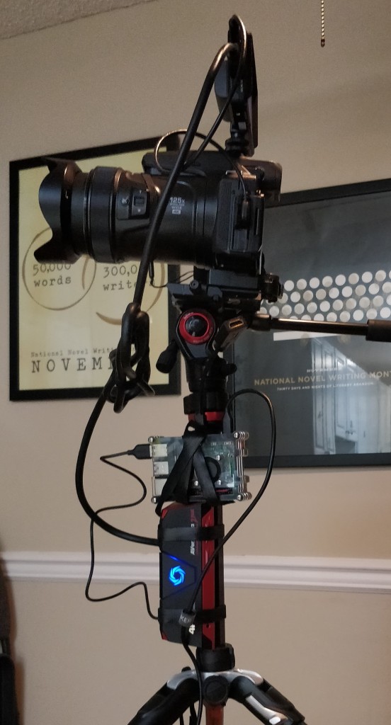
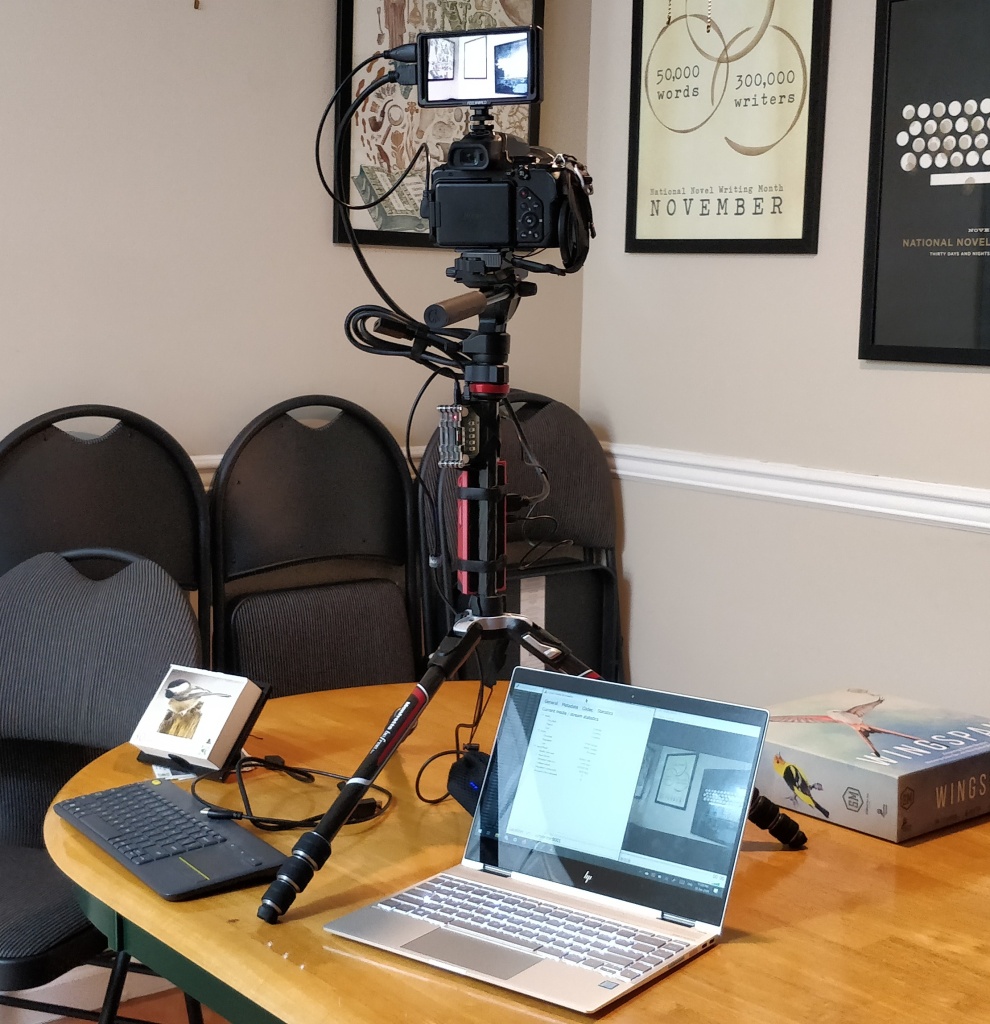
My P1000 with HDMI monitor, connected to the GC513 capture device running from an RPi4 powered by a battery bank over USB. It works!
Putting it all Together
Getting the capture device recognized by Linux was very straightforward. I plugged it in and connected an HDMI input, and Linux instantly recognized it. Getting useful output out of it was a different matter.
The first problem was that the ffmpeg packages that Arch Linux ARM is using don’t have support for the RPi’s built in video encoders, so I needed to compile the package myself and with some out-of-tree patches (that are due to be merged in soon, hopefully).
With a little lot of trial and error, I managed to get the capture device working with a Raspberry Pi at 1080p30, the maximum the RPi4 is rated for. It just barely keeps up, but potentially trans-rating (like transcoding, except changing the bitrate but not fully re-encoding the video) makes things faster. I managed to run a stream for hours without any dropped frames, other than those caused by WiFi glitches.
I tried to get RTMP running well, but it choked on a cellular connection, and even on a good wired ethernet connection, the latency made it unusable for live, real-time video. One thing I did experiment a lot successfully with is using SRT (Secure Reliable Transport) for streaming. Bonus, SRT will be adding bonding soon, claiming this month (Feb. 2020).
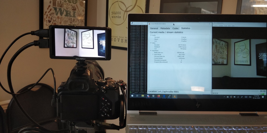
It lives! SRT streaming my dining room wall to VLC on my laptop via my main Linux environment. Dropped frames are from the WiFi, not on the sending end.
Other Things
The streaming on the GoPro Hero 7 Black is unusable. It stops after around an hour no matter what I do and is very annoying to get connected/reconnected, as it needs to use the app. There is a community project to implement an unofficial API, but it doesn’t look like it’ll fix the streaming issue. According to GoPro support it’s a hardware issue, which they won’t fix, instead telling me to buy a Hero 8 Black to replace my broken, but in-warranty 7. Boo.
HDMI switchers, meant to switch in puts on TVs are a bad idea. I bought one model that wasn’t the cheapest, but at best I got about a half second of black screen when it switched over, and at worst, it locked up the HDMI capture device necessitating a replug of the USB, or even needing to power-cycle the RPi4. I looked at higher-end HDMI switchers, but didn’t really find anything mobile, and definitely didn’t find anything inexpensive.
One, Two, N…
There’s a saying in computer circles that getting two of something working is just as much work as getting one of something working. And once you have two working, it as much work to generalize to n.
And it doesn’t have enough decoding power on the RPi4 to decode two streams, switch between them and re-encode them. It just can’t handle that.
Next I tried a custom build of ffmpeg that allows switching between two streams, something stock ffmpeg doesn’t really support. The results were, now that I’m writing this in hindsight, entirely expected. Garbled, unwatchable video for a few seconds until the next I-frame shows up due to smashing unrelated video frames together.
No More Raspberry Pi?
It’s painful to spend so much time on something and realize that it just won’t work out, but between the issues with the RPi4’s encoder just not being powerful enough to do two stream, and a major new issue I uncovered, I’m looking at alternatives.
What major new issue? Well, I was wondering if I could send 2x1080p30 streams at once and calculated how much the data was going to cost me. We’re talking in excess of $80 per hour at Canadian cell phone rates. Oof, so that’s not viable, but even $40 an hour is getting expensive.
I realized that H.264 is years old at this point, and the industry has generally started using H.265 (AKA HEVC). It claims double the efficiency, or better, so I should be able to target a 3Mb/s bitrate for the same quality as H.264’s 6Mb/s. With that in mind I’m trying to find SBCs that support H.265 encoding and have enough decoding performance to work with two streams. It might also be easier to get two raw capture devices, such as Elgato’s Camlink 4k, but this could require a beefy system to do.
I’ve looked at hundreds of boards at this point. Boards based on the RK3288 may work, but the driver situation looks awful. Another potential option is the LattePanda Delta, but it looks too hot and power hungry to be a good contender. There are other similar systems, such as the Atomic Pi, but they look like they may have similar issues with power usage.
So that’s where things are right now. I’m a bit stuck. Sorry RPi4, you’re good for a lot of things, but video isn’t one of them.
Having built a Ceph cluster with three Raspberry Pi 3 B+s and unsuccessfully tested it with RBD, it’s time to try CephFS and Rados Gateway. The cluster setup post is here and the test setup and RBD results post is here. Given how poorly RBD performed, I’m expecting similar poor performance from CephFS. Using the object storage gateway might work better, but I don’t have high hopes for the cluster staying stable under even small loads in either test.
Test Setup:
I’m using the same test setup as I used in the RBD tests. Two pools, one using 2x replication and the other using erasure coding. Test client is an Arch Linux system running a 5.1.14 kernel with Ceph 13.2.1, a quad core CPU, 16GiB of RAM and connected via a 1GbE connection to the cluster. I’m also running the OSDs with their cache limited to 256MiB maximum size, and the metadata cache limited to 128MiB.
CephFS:
CephFS requires a metadata pool, so I created a replicated pool for metadata. Why not create both at once? CephFS doesn’t currently support multiple filesystems on the same cluster, though there is experimental support for it.
With the pool created and the CephFS filesystem mounted on my test client, I started the dd write test with a 12GiB file using dd if=/dev/zero of=/mnt/test/test.dd bs=4M count=3072. The first run completed almost instantly, apparently completely fitting in the filesystem cache. CephFS doesn’t support iflag=direct in dd, so I simply reran the write test knowing that the cache was pretty full at this point. Almost instantly, with less than 1GiB into the test, two of the nodes simultaneously fell over and died. They were completely unreachable over the network, but this time I connected a HDMI monitor to them to see the console. I saw quickly that kthread had been blocked for over 120 seconds, and the system was pretty completely unusable. A USB keyboard was recognized, but key-presses weren’t registering. I power-cycled the systems after waiting at least five minutes, and they came up fine.
A very unhappy Ceph cluster with two hosts that have locked up.
I tried running the test again, and both hosts quickly locked up. I was running top as they did so, and both hosts rapidly consumed their memory. Despite having the OSD’s cache set to a maximum of 256MiB, the ceph-osd process was using around 750MiB before the system became unresponsive. OOM killer didn’t kill cpeh-osd in this case to save the system, possibly due to the kernel failing to allocate memory internally to do so. CephFS seems to hang the Raspberry Pis hard.
I decided to test a bunch of smaller files, because CephFS is meant more as a general filesystem with a bunch of files, whereas RBD tends to get used to store large VM images. I used sysbench to create 1024 16MiB files for a total of 16GiB on my 40GiB CephFS filesystem. Initially, things seemed to work fine. Sysbench reported that it created the 1024 files at 6.4MB/s. While this was just test preparation, it seemed to be a good sign.
What didn’t seem such a good sign was when I actually started running the sysbench write test and Ceph started complaining about slow MDS ops. A lot of them. The sysbench write test immediately failed, citing an IO error on the file. Running ls -la showed a lot of 0 bytes file, with a couple 16MiB files. Ugh. I recreated the test setup, this time with writes at a blazing 540kB/s. When it finally finished several hours later, attempting to run the write tests showed the same truncation of files to 0B as before. This seemed to be a sysbench issue, but I didn’t spend much time troubleshooting it.
For completeness, I also tried an erasure coded pool with CephFS. Like RBD, the metadata pool isn’t supported on erasure coded pools, and needs to be on a replicated pool. Results initially looked better, but the OSDs still exhausted their memory and caused host freezes, though after a longer time with more data successfully ingested.
RadosGW:
I had intended to test RadosGW with the S3 API, but I decided against it. With two different failed tests, the chances for any test results that didn’t end with the cluster dying are pretty low.
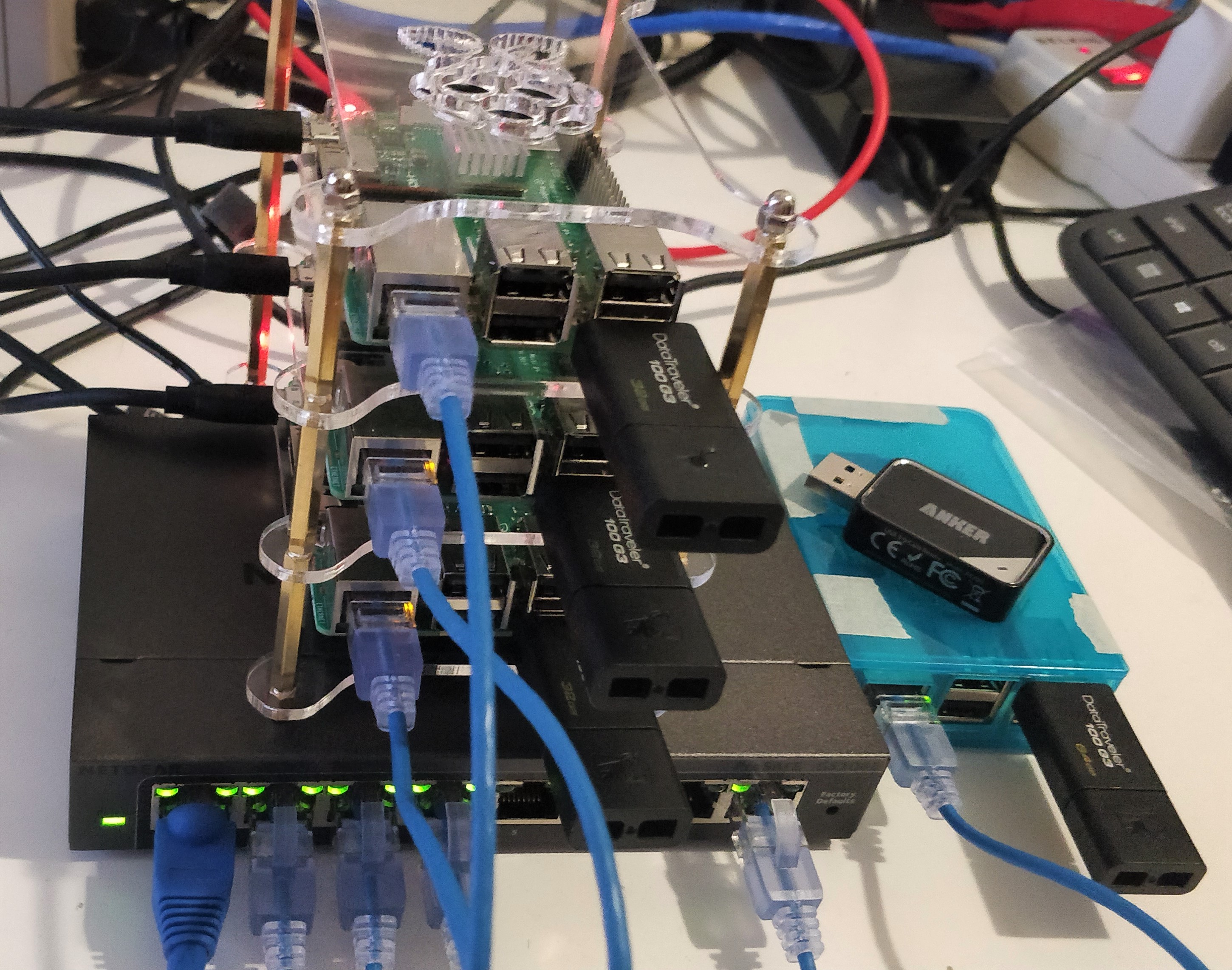
The final cluster hardware setup, with three nodes mounted in a nice stack with shorter (and tidier) network cables. Blue cased Pi isn’t part of the cluster.
Conclusions:
The Raspberry Pi 3 B+ doesn’t have enough RAM to run Ceph. While everything technically works, any attempts at sustained data transfer to or from the cluster fail. It seems like a Raspberry Pi, or other SBC, with 2GB+ of RAM would actually be stable, but still slow. The RAM issue is likely exacerbated by the 900kB/s random write rate the flash keys are capable of, but I don’t have faster flash keys or spare USB hard drives to test with.
Erasure coding seems to be better on RAM limited systems, and while it still failed, it always failed later, with more data successfully written. While it may have been more taxing on the Raspberry Pi’s limited CPU resources, these resources were typically in low contention, with usage averaging around 25% under maximum load across all 4 cores.
The release of the Raspberry Pi 4 B happened while I was writing this series of blog posts. I’d love to re-rerun these tests on three or four of the 4GB models with actual storage drives. The extra RAM should keep the OSDs from running out of memory and dying/taking down the whole system, and the USB3.0 interconnect means that storage and network access will be considerably faster. They might be good enough to run a small, yet stable cluster, and I look forward to testing on them soon.
It’s time to run some tests on the Raspberry Pi Ceph cluster I built. I’m not sure if it’ll be stable enough to actually test, but I’d like to find out and try to tune things if needed.
Pool Creation:
I want to test both standard replicated pools, and Ceph’s newer erasure coded pools. I configured Ceph’s replicated pools with 2 replicas. The erasure coded pools are more like RAID in that there aren’t N replicas spread across the cluster, but rather data is split into chunks and distributed, checksummed, and then the data and checksums are spread across the pool. I configured the erasure coded pool with data split into 2 with an additional coding chunk. Practically, this means that they should tolerate the same failures, but with 1.5x the overhead instead of 2x the overhead.
I created one 16GiB pool of each type to test. Why not always use erasure coded pools? They’re more computationally complex, which might be bad on compute constrained devices such as the Raspberry Pi. They also don’t support the full set of operations. For example, RBD can’t completely reside on an erasure coded pool. There is a workaround, the metadata resides on a replicated pool with the data on the erasure coded pool.
Baseline Tests:
To get a basic idea for what performance level I could expect from the hardware underlying Ceph, I ran network and storage performance tests.
I tested network throughput with iperf between each Raspberry Pi 3 B+ and an external computer connected over Gigabit Ethernet. Each got around 250Mb/s, which is reasonable for a gigabit chip connected via USB2.0. For comparison, a Raspberry Pi 3 B (not the plus version) with Fast Ethernet tested around 95Mb/s. As a control, I also tested the same iperf client against another computer connected over full gigabit at 950Mb/s.
Disk throughput was tested usingdd for sequential reads and writes and iometer for random reads and writes against a flash key with an XFS filesystem. XFS used to be the recommended filesystem for Ceph until Ceph released BlueStore, and it’s still used for BlueStore’s metadata storage partition. The 32GB flash keys performed at 32.7MB/s sequential read and 16.5 MB/s sequential write. Random read and write with 16kiB operations yielded 15MB/s and 0.9MB/s (that’s 900kB/s) respectively using sysbench’s fileio module.
RBD Tests:
RADOS Block Device (RBD) is a block storage service, so you can run your own filesystem but have Ceph’s replication protect the data as well as spread access over multiple drives for increased performance. Ceph currently doesn’t support using pure erasure coded pools for RBD (or CephFS), instead the data is stored in the erasure coded pool and the metedata in a replicated pool. Partial writes also need to be enabled per-pool, as per the docs.
Once the pools were created, I mounted each and started running tests. The first thing I wanted to test was just sequential read and write of data. To do this, I made an XFS filesystem with the defaults and mounted it on a test client (Arch Linux, kernel 5.1.14, quad core, 16GiB RAM, 1xGbE, Ceph 13.2.1) and wrote a file using dd if=/dev/zero of=/mnt/test/test.dd bs=4M count=3072 iflag=direct. Initially, writes to the replicated rbd image looked decent, averaging a whopping 6.4MB/s. And then the VM suddenly got really cranky.
The Ceph manager dashboard’s health status. Not what I’d been hoping for during a performance test.
One host, rpi-node2 had seemingly dropped from the network. Ceph went into recovery mode to keep my precious zeroes intact, and IO basically ground to a halt as the cluster recovered at a blazing 1.3MiB/s. I couldn’t hit the node with SSH, so I power-cycled it. It came back up, Ceph realized that the OSD was back and cut short the re-balancing of the cluster. I decided to run the write test again, deleted the test file and ran fstrim -v /mnt/test, which tells Ceph that the blocks can be freed, so it frees up that space on the OSDs so I could re-run fresh.
The second test ended similarly to the first, with dd writing happily at 6.1MB/s until rpi-node3 stopped responding (including to SSH) at 3.9GB written. This time I stopped dd immediately and waited for the node to come back, which is did after almost two minutes. I checked the logs and saw that the system was running out of memory and the ceph-osd process was getting OOM killed. I also noticed that both nodes that had failed were the ones running the active ceph-mgr instance serving the dashboards.
I ran the test again, this time generating a 1GiB file instead and confirmed that it was the node with the ceph-mgs instance running out of memory. I also let the write finish, testing how well Ceph ran in the degraded state. At 2.8MB/s, no performance records were being set, but the cluster was still ingesting data with one node missing.
I have two options, the first is to move the ceph-mgr daemon to another device, but as I wanted the cluster to be self-contained to three nodes, so I opted for the second option. Option two is to lower the memory usage of the ceph-osd daemon. I looked at the documentation for the BlueStore config, and saw that the default cache size is 1 GiB, or as much RAM as the Pi has. That just won’t do, so I added bluestore_cache_size = 536870912 and bluestore_cache_kv_max = 268435456 to my ceph.conf file and restarted the OSDs. This means that BlueStore will use at most 512MiB of RAM for its caches with only 256MiB maximum for the RocksDB metadata cache.
I reran the 1GiB file test and had 3.5M B/s write speed and no OSDs getting killed. With the 16GiB file, writes averaged 3MB/s, but RAM usage at the halfway mark eventually got the OSD running on the same node as the active ceph-mgr killed. Again, the cluster survived, just in a less happy state until the killed OSD daemon restarted. I disabled the dashboard, and while this helped RAM usage, the ceph-osd daemon was still getting killed. I further dropped the BlueStore cache to 256MiB and 128MiB for the metadata store. This time I locked two of the three nodes up hard and needed to power-cycle them.
During the 1GiB file tests, this was the unhappiest the cluster got. The PGs were simply being slow replicating and caught up quickly once the write load subsided.
With the replicated testing being close to a complete failure, I moved on to testing the erasure coded pool. I expected them to be worse due the the increased amount of compute resources needed. I was wrong. I was able to successfully write the test file, and the worst I got was an OSD being slow and not responding to the the monitor fast enough and then recovering a few seconds later. Sequential writes averaged 5.7MB/s and sequential read was an average of 6.1MB/s, but I still had two nodes go down at different times. It seems that erasure coded pools perform slightly better, but can still cause system memory exhaustion.
One thing to note is that even with three nodes, Ceph never lost any data and was still accepting write, just very slowly. I hadn’t intended to test Ceph’s resiliency, as that has already been well tested, but it was nice to see that it kept serving reads and writes.
At this point, I don’t think that the 1GiB of RAM is enough to run RBD properly. Sequential writes looked to be around 6MB/s when the cluster hadn’t lost any OSDs or whole hosts. I never attempted to test random access, due to the issues with sequential reads and writes.
CephFS and Rados Gateway:
With RBD being a bit of a bust, I wanted to see if CephFS and Rados Gateway performed better. As this post is getting long, CephFS and RadosGW results are in a second post, along with a conclusion.
One of the more recent tools I’ve added to my repertoire for reverse engineering the game simulation is inspecting the memory of a running game to see how things vary without needing to pause the game and count individual tiles in the game many times.
Power Plants and Cheat Engine:
To calculate the MW rating for power plants to tiles powered I could have built a city and connected a power plant to it and then counted the number of powered tiles, but the game has a variable that stores the total power produced. I could just build a city and look at this value, swapping power plants out as needed.
My go to tool for finding, viewing (and sometimes editing) values in memory is Cheat Engine. I use it to search for a known value, pulled from the save file, and then I get the value at that memory location. SC2k always uses the same memory addresses each time it starts up, so I slowly built up a table of where memory locations end up, at least for the common stuff.
Why didn’t I just build the plant, pause, save, load it into my parser and look at the value? Memory inspection is way faster after the initial discovery, and allowed me to more rapidly test other things.
Cheat Engine address table showing some of the interesting addressed. The total amount of power produced is highlighted.
Once I found the total power variable, it was pretty quick to calculate that the MW rating for power plants doesn’t actually mean anything and each power plant has an internal statistic for how many tiles it powers, including the tiles that make up the plant itself!
For more info, see the spec here.
Weather – Beyond Cheat Engine:
But what happens when I want to look at the correlation between various values over many game cycles? Does weather, specifically temperature, affect the crime rate? If so, how much? Weather definitely affects how much electricity solar and wind power plants produce as well as how much water is pumped, but what’s the formula there?
Basically, how do I get those values from the running game and make decisions on it?
I’m still working on answering that question, but at it’s most basic level, I want to read various memory values once per tick of the game. The tick count is also used to determine the date of the game, which starts at a certain epoch.
So I wrote a simple python program the dumps values at memory locations once per game tick and another that uses pandas, numpy and matplotlib to do some analysis.
For power plants, I didn’t need anything fancy. I could see by quick inspection of values that wind power is indeed strongly affected by altitude and to a lesser extent how windy it is. Solar power is also affected by how humid it is, but both also have a random component involved. The simulation specification documents show how the weather affects wind and solar power in greater detail.
But what does this “look” like? I logged several hundred thousand values and created a correlation graph using numpy, pandas and matplotlib and a city containing a single power plant and a single water pump.
Correlation between (solar) power and water production.
What’s this graph telling us? Well, solar power production is negatively correlated with how humid (-0.298) and windy (-0.245) it is. Not knowing exactly what this represents in the game, it seems that higher values are probably rainier. I didn’t bin the weather the same way, as the game treats it like discrete values rather than the “continuous” values for humidity and windiness. So solar power is definitely affected by weather. On the other hand, it looks like water production is positively impacted by the weather (0.486 correlation with humidity and 0.242 with windiness) which seems like in rainy weather pumps produces more water. This is about what the game does.
But what about crime? Below is a correlation graph generated the same way.
Correlation between crime and various game weather variables. The diagonal line are how much a thing correlates with itself, which is always 1.0 or completely correlated, as expected.
So what sort of correlation do we see between crime and how hot it is? Almost none, but there is a slight correlation, 0.0287, so it does affect the simulation a little bit. Unsurprisingly, the type of weather is well correlated with wind (0.525), humidity (0.877) and heat (0.287). This isn’t enough to know how the formula works, because there is randomness at work, but it’s a start to figuring it out.
I’m not sure if this sort of analysis is actually going to be useful working to reverse engineer the game, but it’s definitely a useful place to get started, and may yet be a useful tool to determine exactly what is happening internal to the simulation.